Exercises
Exercise 1: Quantum Dice
Write a quantum program to simulate throwing an 8-sided die. The Python function you should produce is:
def throw_octahedral_die():
    # return the result of throwing an 8 sided die, an int between 1 and 8, by running a quantum program
Next, extend the program to work for any kind of fair die:
def throw_polyhedral_die(num_sides):
    # return the result of throwing a num_sides sided die by running a quantum program
Exercise 2: Controlled Gates
We can use the full generality of NumPy to construct new gate matrices.
Write a function
controlledwhich takes a \(2\times 2\) matrix \(U\) representing a single qubit operator, and makes a \(4\times 4\) matrix which is a controlled variant of \(U\), with the first argument being the control qubit.Write a Quil program to define a controlled-\(Y\) gate in this manner. Find the wavefunction when applying this gate to qubit 1 controlled by qubit 0.
Exercise 3: Grover’s Algorithm
Write a quantum program for the single-shot Grover’s algorithm. The Python function you should produce is:
# data is an array of 0's and 1's such that there are exactly three times as many
# 0's as 1's
def single_shot_grovers(data):
    # return an index that contains the value 1
As an example: single_shot_grovers([0,0,1,0]) should return 2.
HINT - Remember that the Grover’s diffusion operator is:
Exercise 4: Prisoner’s Dilemma
A classic strategy game is the prisoner’s dilemma where two prisoners get the minimal penalty if they collaborate and stay silent, get zero penalty if one of them defects and the other collaborates (incurring maximum penalty) and get intermediate penalty if they both defect. This game has an equilibrium where both defect and incur intermediate penalty.
However, things change dramatically when we allow for quantum strategies leading to the Quantum Prisoner’s Dilemma.
Can you design a program that simulates this game?
Exercise 5: Quantum Fourier Transform
The quantum Fourier transform (QFT) is a quantum implementation of the discrete Fourier transform. The Fourier transform can be used to transform a function from the time domain into the frequency domain.
- Compute the discrete Fourier transform of
[0, 1, 0, 0, 0, 0, 0, 0], using pyQuil: Write a state preparation quantum program.
Write a function to make a 3-qubit QFT program, taking qubit indices as arguments.
Combine your solutions to part a and b into one program and use the
WavefunctionSimulatorto get the solution.
Note
For a more challenging initial state, try 01100100.
Solution
Part a: Prepare the initial state
We are going to apply the QFT on the amplitudes of the states.
We want to prepare a state that corresponds to the sequence for which we want to compute the discrete Fourier transform. As the exercise hinted in part b, we need 3 qubits to transform an 8 bit sequence. It is simplest to understand if we think of the qubits as three digits in a binary string (aka bitstring). There are 8 possible values the bitstring can have, and in our quantum state, each of these possibilities has an amplitude. Our 8 indices in the QFT sequence label each of these states. For clarity:
\(|000\rangle\) => 10000000
\(|001\rangle\) => 01000000
…
\(|111\rangle\) -> 00000001
The sequence we want to compute is 01000000, so our initial state is simply \(|001\rangle\). For a bitstring with more
than one 1, we would want an equal superposition over all the selected states. (E.g. 01100000 would be an
equal superposition of \(|001\rangle\) and \(|010\rangle\)).
To set up the \(|001\rangle\) state, we only have to apply one \(X\)-gate to the zeroth qubit.
from pyquil import Program
from pyquil.gates import *

state_prep = Program(X(0))
We can verify that this works by computing its wavefunction with the
Wavefunction Simulator. However, we need to add some “dummy” qubits,
because otherwise wavefunction would return a two-element vector for only qubit 0.
from pyquil.api import WavefunctionSimulator

add_dummy_qubits = Program(I(1), I(2))  # The identity gate I has no effect

wf_sim = WavefunctionSimulator()
wavefunction = wf_sim.wavefunction(state_prep + add_dummy_qubits)
print(wavefunction)
(1+0j)|001>
We’ll need wf_sim for part c, too.
Part b: Three qubit QFT program
In this part, we define a function, qft3, to make a 3-qubit QFT quantum program. The algorithm
is nicely described on this page.
It is a mix of Hadamard and CPHASE gates, with a SWAP gate for bit reversal correction.
from math import pi

def qft3(q0, q1, q2):
    p = Program()
    p += [SWAP(q0, q2),
          H(q0),
          CPHASE(-pi / 2.0, q0, q1),
          H(q1),
          CPHASE(-pi / 4.0, q0, q2),
          CPHASE(-pi / 2.0, q1, q2),
          H(q2)]
    return p
There is a very important detail to recognize here: The function
qft3 doesn’t compute the QFT, but rather it makes a quantum
program to compute the QFT on qubits q0, q1, and q2.
We can see what this program looks like in Quil notation with print(qft(0, 1, 2)).
SWAP 0 2
H 0
CPHASE(-1.5707963267948966) 0 1
H 1
CPHASE(-0.7853981633974483) 0 2
CPHASE(-1.5707963267948966) 1 2
H 2
Part c: Execute the QFT
Combining parts a and b:
compute_qft_prog = state_prep + qft3(0, 1, 2)
wavefunction = wf_sim.wavefunction(compute_qft_prog)
print(wavefunction.amplitudes)
[ 3.53553391e-01+0.j          2.50000000e-01-0.25j
  2.16489014e-17-0.35355339j -2.50000000e-01-0.25j
 -3.53553391e-01+0.j         -2.50000000e-01+0.25j
 -2.16489014e-17+0.35355339j  2.50000000e-01+0.25j      ]
We can verify this works by computing the inverse FFT on the output with NumPy and seeing that we get back our input (with some floating point error).
from numpy.fft import ifft
print(ifft(wavefunction.amplitudes, norm="ortho"))
[ 0.00000000e+00+0.00000000e+00j  1.00000000e+00+5.45603965e-17j
  0.00000000e+00+0.00000000e+00j  0.00000000e+00-1.53080850e-17j
  0.00000000e+00+0.00000000e+00j -7.85046229e-17-2.39442265e-17j
  0.00000000e+00+0.00000000e+00j  0.00000000e+00-1.53080850e-17j]
After ignoring the terms that are on the order of 1e-17, we get [0, 1, 0, 0, 0, 0, 0, 0], which was our input!
Example: The Meyer-Penny Game
To create intuition for quantum algorithms, it is useful (and fun) to play with the abstraction that the software provides.
The Meyer-Penny Game [1] is a simple example we’ll use from quantum game theory. The interested reader may want to read more about quantum game theory in the article Toward a general theory of quantum games [2]. The Meyer-Penny Game goes as follows:
The Starship Enterprise, during one of its deep-space missions, is facing an immediate calamity at the edge of a wormhole, when a powerful alien suddenly appears. The alien, named Q, offers to help Picard, the captain of the Enterprise, under the condition that Picard beats Q in a simple game of heads or tails.
The rules
Picard is to place a penny heads up into an opaque box. Then Picard and Q take turns to flip or not flip the penny without being able to see it; first Q then P then Q again. After this the penny is revealed; Q wins if it shows heads (H), while tails (T) makes Picard the winner.
Picard vs. Q
Picard quickly estimates that his chance of winning is 50% and agrees to play the game. He loses the first round and insists on playing again. To his surprise Q agrees, and they continue playing several rounds more, each of which Picard loses. How is that possible?
What Picard did not anticipate is that Q has access to quantum tools. Instead of flipping the penny, Q puts the penny into a superposition of heads and tails proportional to the quantum state \(|H\rangle+|T\rangle\). Then no matter whether Picard flips the penny or not, it will stay in a superposition (though the relative sign might change). In the third step Q undoes the superposition and always finds the penny to show heads.
Let’s see how this works!
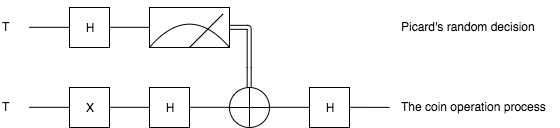
To simulate the game we first construct the corresponding quantum circuit, which takes two qubits: one to simulate Picard’s choice whether or not to flip the penny, and the other to represent the penny. The initial state for all qubits is \(|0\rangle\) (which is mapped to \(|T\rangle\), tails). To simulate Picard’s decision, we assume that he chooses randomly whether or not to flip the coin, in agreement with the optimal strategy for the classic penny-flip game. This random choice can be created by putting one qubit into an equal superposition, e.g. with the Hadamard gate \(H\), and then measure its state. The measurement will show heads or tails with equal probability \(p_h=p_t=0.5\).
To simulate the penny flip game we take the second qubit and put it into its excited state \(|1\rangle\) (which is mapped to \(|H\rangle\), heads) by applying the X (or NOT) gate. Q’s first move is to apply the Hadamard gate H. Picard’s decision about the flip is simulated as a CNOT operation where the control bit is the outcome of the random number generator described above. Finally Q applies a Hadamard gate again, before we measure the outcome. The full circuit is shown in the figure below.
In pyQuil
We first import and initialize the necessary tools [3]
from pyquil import Program
from pyquil.api import WavefunctionSimulator
from pyquil.gates import *

wf_sim = WavefunctionSimulator()
p = Program()
and then wire it all up into the overall measurement circuit; remember that qubit 0 is the penny, and qubit 1 represents Picard’s choice.
p += X(0)
p += H(0)
p += H(1)
p += CNOT(1, 0)
p += H(0)
We use the quantum mechanics principle of deferred measurement to keep all the measurement logic separate from the gates.
Our method call to the WavefunctionSimulator will handle measuring for us [4].
Finally, we play the game several times. (Remember to run your qvm server.)
results = wf_sim.run_and_measure(p, trials=10)
print(results)
[[1 1]
 [1 1]
 [1 1]
 [1 1]
 [1 1]
 [1 0]
 [1 1]
 [1 1]
 [1 1]
 [1 0]]
In each trial, the first number is the outcome of the game, whereas the second number represents Picard’s choice to flip or not flip the penny.
Inspecting the results, we see that no matter what Picard does, Q will always win!