Noise and quantum computation
Modeling noisy quantum gates
Pure states vs. mixed states
Errors in quantum computing can introduce classical uncertainty in what the underlying state is. When this happens we sometimes need to consider not only wavefunctions but also probabilistic sums of wavefunctions when we are uncertain as to which one we have. For example, if we think that an X gate was accidentally applied to a qubit with a 50-50 chance then we would say that there is a 50% chance we have the \(\ket{0}\) state and a 50% chance that we have a \(\ket{1}\) state. This is called an “impure” or “mixed”state in that it isn’t just a wavefunction (which is pure) but instead a distribution over wavefunctions. We describe this with something called a density matrix, which is generally an operator. Pure states have very simple density matrices that we can write as an outer product of a ket vector \(\ket{\psi}\) with its own bra version \(\bra{\psi}=\ket{\psi}^\dagger\). For a pure state the density matrix is simply
The expectation value of an operator for a mixed state is given by
where \(\tr{\cdot}\) is the trace of an operator, which is the sum of its diagonal elements, which is independent of choice of basis. Pure state density matrices satisfy
which you can easily verify for \(\rho_\psi\) assuming that the state is normalized. If we want to describe a situation with classical uncertainty between states \(\rho_1\) and \(\rho_2\), then we can take their weighted sum
where \(p\in [0,1]\) gives the classical probability that the state is \(\rho_1\).
Note that classical uncertainty in the wavefunction is markedly different from superpositions. We can represent superpositions using wavefunctions, but use density matrices to describe distributions over wavefunctions. You can read more about density matrices here [DensityMatrix].
Quantum Gate Errors
For a quantum gate given by its unitary operator \(U\), a “quantum gate error” describes the scenario in which the actually induced transformation deviates from \(\ket{\psi} \mapsto U\ket{\psi}\). There are two basic types of quantum gate errors:
coherent errors are those that preserve the purity of the input state, i.e., instead of the above mapping we carry out a perturbed, but unitary operation \(\ket{\psi} \mapsto \tilde{U}\ket{\psi}\), where \(\tilde{U} \neq U\).
incoherent errors are those that do not preserve the purity of the input state, in this case we must actually represent the evolution in terms of density matrices. The state \(\rho := \ket{\psi}\bra{\psi}\) is then mapped as
\[\rho \mapsto \sum_{j=1}^m K_j\rho K_j^\dagger,\]where the operators \(\{K_1, K_2, \dots, K_m\}\) are called Kraus operators and must obey \(\sum_{j=1}^m K_j^\dagger K_j = I\) to conserve the trace of \(\rho\). Maps expressed in the above form are called Kraus maps. It can be shown that every physical map on a finite dimensional quantum system can be represented as a Kraus map, though this representation is not generally unique. You can find more information about quantum operations here
In a way, coherent errors are in principle amendable by more precisely calibrated control. Incoherent errors are more tricky.
Why do incoherent errors happen?
When a quantum system (e.g., the qubits on a quantum processor) is not perfectly isolated from its environment it generally co-evolves with the degrees of freedom it couples to. The implication is that while the total time evolution of system and environment can be assumed to be unitary, restriction to the system state generally is not.
Let’s throw some math at this for clarity: Let our total Hilbert space be given by the tensor product of system and environment Hilbert spaces: \(\mathcal{H} = \mathcal{H}_S \otimes \mathcal{H}_E\). Our system “not being perfectly isolated” must be translated to the statement that the global Hamiltonian contains a contribution that couples the system and environment:
where \(V\) non-trivally acts on both the system and the environment. Consequently, even if we started in an initial state that factorized over system and environment \(\ket{\psi}_{S,0}\otimes \ket{\psi}_{E,0}\) if everything evolves by the Schrödinger equation
the final state will generally not admit such a factorization.
A toy model
In this (somewhat technical) section we show how environment interaction can corrupt an identity gate and derive its Kraus map. For simplicity, let us assume that we are in a reference frame in which both the system and environment Hamiltonian’s vanish \(H_S = 0, H_E = 0\) and where the cross-coupling is small even when multiplied by the duration of the time evolution \(\|\frac{tV}{\hbar}\|^2 \sim \epsilon \ll 1\) (any operator norm \(\|\cdot\|\) will do here). Let us further assume that \(V = \sqrt{\epsilon} V_S \otimes V_E\) (the more general case is given by a sum of such terms) and that the initial environment state satisfies \(\bra{\psi}_{E,0} V_E\ket{\psi}_{E,0} = 0\). This turns out to be a very reasonable assumption in practice but a more thorough discussion exceeds our scope.
Then the joint system + environment state \(\rho = \rho_{S,0} \otimes \rho_{E,0}\) (now written as a density matrix) evolves as
Using the Baker-Campbell-Hausdorff theorem we can expand this to second order in \(\epsilon\)
We can insert the initially factorizable state \(\rho = \rho_{S,0} \otimes \rho_{E,0}\) and trace over the environmental degrees of freedom to obtain
where the coefficient in front of the second part is by our initial assumption very small \(\gamma := \frac{\epsilon t^2}{2\hbar^2}\tr{V_E^2 \rho_{E,0}} \ll 1\). This evolution happens to be approximately equal to a Kraus map with operators \(K_1 := I - \frac{\gamma}{2} V_S^2, K_2:= \sqrt{\gamma} V_S\):
This agrees to \(O(\epsilon^{3/2})\) with the result of our derivation above. This type of derivation can be extended to many other cases with little complication and a very similar argument is used to derive the Lindblad master equation.
Noisy gates on the QVM
As of today, users of the Quil SDK can annotate their Quil programs by certain pragma statements that inform the QVM that a particular gate on specific target qubits should be replaced by an imperfect realization given by a Kraus map.
The QVM propagates pure states — so how does it simulate noisy gates? It does so by yielding the correct outcomes in the average over many executions of the Quil program: When the noisy version of a gate should be applied the QVM makes a random choice which Kraus operator is applied to the current state with a probability that ensures that the average over many executions is equivalent to the Kraus map. In particular, a particular Kraus operator \(K_j\) is applied to \(\ket{\psi}_S\)
with probability \(p_j:= \bra{\psi}_S K_j^\dagger K_j \ket{\psi}_S\). In the average over many execution \(N \gg 1\) we therefore find that
where \(j_n\) is the chosen Kraus operator label in the \(n\)-th trial. This is clearly a Kraus map itself! And we can group identical terms and rewrite it as
where \(N_{\ell}\) is the number of times that Kraus operator label \(\ell\) was selected. For large enough \(N\) we know that \(N_{\ell} \approx N p_\ell\) and therefore
which proves our claim. The consequence is that noisy gate simulations must generally be repeated many times to obtain representative results.
Getting started
Come up with a good model for your noise. We will provide some examples below and may add more such examples to our public repositories over time. Alternatively, you can characterize the gate under consideration using Quantum Process Tomography or Gate Set Tomography and use the resulting process matrices to obtain a very accurate noise model for a particular QPU.
Define your Kraus operators as a list of numpy arrays
kraus_ops = [K1, K2, ..., Km].For your Quil program
p, call:p.define_noisy_gate("MY_NOISY_GATE", [q1, q2], kraus_ops)
where you should replace
MY_NOISY_GATEwith the gate of interest andq1, q2with the indices of the qubits.
Scroll down for some examples!
import matplotlib.colors as colors
import matplotlib.pyplot as plt
import numpy as np

from pyquil import Program, get_qc
from pyquil.gates import CZ, H, I, X, MEASURE
from pyquil.quilbase import Declare
from scipy.linalg import expm
from scipy.stats import binom
# We could ask for "2q-noisy-qvm" but we will be specifying
# our noise model as PRAGMAs on the Program itself.
qc = get_qc('2q-qvm')
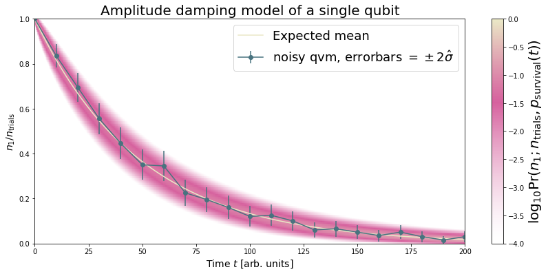
Example 1: Amplitude damping
Amplitude damping channels are imperfect identity maps with Kraus operators
where \(p\) is the probability that a qubit in the \(\ket{1}\) state decays to the \(\ket{0}\) state.
def damping_channel(damp_prob=.1):
    """
    Generate the Kraus operators corresponding to an amplitude damping
    noise channel.

    :params float damp_prob: The one-step damping probability.
    :return: A list [k1, k2] of the Kraus operators that parametrize the map.
    :rtype: list
    """
    damping_op = np.sqrt(damp_prob) * np.array([[0, 1],
                                                [0, 0]])

    residual_kraus = np.diag([1, np.sqrt(1-damp_prob)])
    return [residual_kraus, damping_op]

def append_kraus_to_gate(kraus_ops, g):
    """
    Follow a gate `g` by a Kraus map described by `kraus_ops`.

    :param list kraus_ops: The Kraus operators.
    :param numpy.ndarray g: The unitary gate.
    :return: A list of transformed Kraus operators.
    """
    return [kj.dot(g) for kj in kraus_ops]


def append_damping_to_gate(gate, damp_prob=.1):
    """
    Generate the Kraus operators corresponding to a given unitary
    single qubit gate followed by an amplitude damping noise channel.

    :params np.ndarray|list gate: The 2x2 unitary gate matrix.
    :params float damp_prob: The one-step damping probability.
    :return: A list [k1, k2] of the Kraus operators that parametrize the map.
    :rtype: list
    """
    return append_kraus_to_gate(damping_channel(damp_prob), gate)
# single step damping probability
damping_per_I = 0.02

# number of program executions
trials = 200

results_damping = []
lengths = np.arange(0, 201, 10, dtype=int)
for jj, num_I in enumerate(lengths):
    p = Program(
        Declare("ro", "BIT", 1),
        X(0),
    )
    # want increasing number of I-gates
    p.inst([I(0) for _ in range(num_I)])
    p.inst(MEASURE(0, ("ro", 0)))

    # overload identity I on qc 0
    p.define_noisy_gate("I", [0], append_damping_to_gate(np.eye(2), damping_per_I))
    p.wrap_in_numshots_loop(trials)
    qc.qam.random_seed = int(num_I)
    res = qc.run(p).get_register_map().get("ro")
    results_damping.append([np.mean(res), np.std(res) / np.sqrt(trials)])

results_damping = np.array(results_damping)
dense_lengths = np.arange(0, lengths.max()+1, .2)
survival_probs = (1-damping_per_I)**dense_lengths
logpmf = binom.logpmf(np.arange(trials+1)[np.newaxis, :], trials, survival_probs[:, np.newaxis])/np.log(10)
DARK_TEAL = '#48737F'
FUSCHIA = "#D6619E"
BEIGE = '#EAE8C6'
cm = colors.LinearSegmentedColormap.from_list('anglemap', ["white", FUSCHIA, BEIGE], N=256, gamma=1.5)
plt.figure(figsize=(14, 6))
plt.pcolor(dense_lengths, np.arange(trials+1)/trials, logpmf.T, cmap=cm, vmin=-4, vmax=logpmf.max())
plt.plot(dense_lengths, survival_probs, c=BEIGE, label="Expected mean")
plt.errorbar(lengths, results_damping[:,0], yerr=2*results_damping[:,1], c=DARK_TEAL,
             label=r"noisy qvm, errorbars $ = \pm 2\hat{\sigma}$", marker="o")
cb = plt.colorbar()
cb.set_label(r"$\log_{10} \mathrm{Pr}(n_1; n_{\rm trials}, p_{\rm survival}(t))$", size=20)

plt.title("Amplitude damping model of a single qubit", size=20)
plt.xlabel(r"Time $t$ [arb. units]", size=14)
plt.ylabel(r"$n_1/n_{\rm trials}$", size=14)
plt.legend(loc="best", fontsize=18)
plt.xlim(*lengths[[0, -1]])
plt.ylim(0, 1)
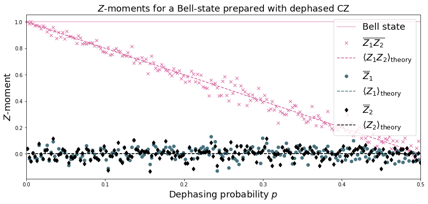
Example 2: Dephased CZ-gate
Dephasing is usually characterized through a qubit’s \(T_2\) time. For a single qubit the dephasing Kraus operators are
where \(p = (1 - \exp(-T_{\rm gate}/T_2))/2\) is the probability that the qubit is dephased over the time interval of interest, \(I_2\) is the \(2\times 2\)-identity matrix and \(\sigma_Z\) is the Pauli-Z operator.
For two qubits, we must construct a Kraus map that has four different outcomes:
No dephasing
Qubit 1 dephases
Qubit 2 dephases
Both dephase
The Kraus operators for this are given by
where we assumed a dephasing probability \(p\) for the first qubit and \(q\) for the second.
Dephasing is a diagonal error channel and the CZ gate is also diagonal, therefore we can get the combined map of dephasing and the CZ gate simply by composing \(U_{\rm CZ}\) the unitary representation of CZ with each Kraus operator
Note that this is not always accurate, because a CZ gate is often achieved through non-diagonal interaction Hamiltonians! However, for sufficiently small dephasing probabilities it should always provide a good starting point.
def dephasing_kraus_map(p=.1):
    """
    Generate the Kraus operators corresponding to a dephasing channel.

    :params float p: The one-step dephasing probability.
    :return: A list [k1, k2] of the Kraus operators that parametrize the map.
    :rtype: list
    """
    return [np.sqrt(1-p)*np.eye(2), np.sqrt(p)*np.diag([1, -1])]

def tensor_kraus_maps(k1, k2):
    """
    Generate the Kraus map corresponding to the composition
    of two maps on different qubits.

    :param list k1: The Kraus operators for the first qubit.
    :param list k2: The Kraus operators for the second qubit.
    :return: A list of tensored Kraus operators.
    """
    return [np.kron(k1j, k2l) for k1j in k1 for k2l in k2]
# single step damping probabilities
ps = np.linspace(.001, .5, 200)

# number of program executions
trials = 500

results = []

for jj, p in enumerate(ps):

    corrupted_CZ = append_kraus_to_gate(
    tensor_kraus_maps(
        dephasing_kraus_map(p),
        dephasing_kraus_map(p)
    ),
    np.diag([1, 1, 1, -1]))

    # make Bell-state
    p = Program(
        Declare("ro", "BIT", 2),
        H(0),
        H(1),
        CZ(0, 1),
        H(1),
    )

    p.inst(MEASURE(0, ("ro", 0)))
    p.inst(MEASURE(1, ("ro", 1)))

    # overload CZ on qc 0
    p.define_noisy_gate("CZ", [0, 1], corrupted_CZ)
    p.wrap_in_numshots_loop(trials)
    qc.qam.random_seed = jj
    res = qc.run(p).get_register_map().get("ro")
    results.append(res)

results = np.array(results)
Z1s = (2*results[:,:,0]-1.)
Z2s = (2*results[:,:,1]-1.)
Z1Z2s = Z1s * Z2s

Z1m = np.mean(Z1s, axis=1)
Z2m = np.mean(Z2s, axis=1)
Z1Z2m = np.mean(Z1Z2s, axis=1)
plt.figure(figsize=(14, 6))
plt.axhline(y=1.0, color=FUSCHIA, alpha=.5, label="Bell state")

plt.plot(ps, Z1Z2m, "x", c=FUSCHIA, label=r"$\overline{Z_1 Z_2}$")
plt.plot(ps, 1-2*ps, "--", c=FUSCHIA, label=r"$\langle Z_1 Z_2\rangle_{\rm theory}$")

plt.plot(ps, Z1m, "o", c=DARK_TEAL, label=r"$\overline{Z}_1$")
plt.plot(ps, 0*ps, "--", c=DARK_TEAL, label=r"$\langle Z_1\rangle_{\rm theory}$")

plt.plot(ps, Z2m, "d", c="k", label=r"$\overline{Z}_2$")
plt.plot(ps, 0*ps, "--", c="k", label=r"$\langle Z_2\rangle_{\rm theory}$")

plt.xlabel(r"Dephasing probability $p$", size=18)
plt.ylabel(r"$Z$-moment", size=18)
plt.title(r"$Z$-moments for a Bell-state prepared with dephased CZ", size=18)
plt.xlim(0, .5)
plt.legend(fontsize=18)
Adding Decoherence Noise
In this example, we investigate how a program might behave on a
near-term device that is subject to T1- and T2-type noise using the convenience function
pyquil.noise.add_decoherence_noise(). The same module also contains some other useful
functions to define your own types of noise models, e.g.,
pyquil.noise.tensor_kraus_maps() for generating multi-qubit noise processes,
pyquil.noise.combine_kraus_maps() for describing the succession of two noise processes and
pyquil.noise.append_kraus_to_gate() which allows appending a noise process to a unitary
gate.
from pyquil.quil import Program
from pyquil.paulis import PauliSum, PauliTerm, exponentiate, exponential_map, trotterize
from pyquil.gates import MEASURE, H, Z, RX, RZ, CZ
from pyquil.quilbase import Declare
import numpy as np
The Task
We want to prepare \(e^{i \theta XY}\) and measure it in the \(Z\) basis.
from numpy import pi
theta = pi/3
xy = PauliTerm('X', 0) * PauliTerm('Y', 1)
The idiomatic pyQuil program
prog = exponential_map(xy)(theta)
print(prog)
H 0
RX(1.5707963267948966) 1
CNOT 0 1
RZ(2.0943951023931953) 1
CNOT 0 1
H 0
RX(-1.5707963267948966) 1
The compiled program
To run on a real device, we must compile each program to the native gate set for the device. The high-level noise model is similarly constrained to use a small, native gate set. In particular, we can use
\(I\)
\(RZ(\theta)\)
\(RX(\pm \pi/2)\)
\(CZ\)
For simplicity, the compiled program is given below but generally you will want to use a compiler to do this step for you.
def get_compiled_prog(theta):
    return Program([
        RZ(-pi/2, 0),
        RX(-pi/2, 0),
        RZ(-pi/2, 1),
        RX( pi/2, 1),
        CZ(1, 0),
        RZ(-pi/2, 1),
        RX(-pi/2, 1),
        RZ(theta, 1),
        RX( pi/2, 1),
        CZ(1, 0),
        RX( pi/2, 0),
        RZ( pi/2, 0),
        RZ(-pi/2, 1),
        RX( pi/2, 1),
        RZ(-pi/2, 1),
    ])
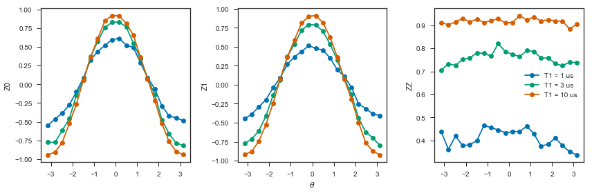
Scan over noise parameters
We perform a scan over three levels of noise, each at 20 theta points.
Specifically, we investigate T1 values of 1, 3, and 10 us. By default, T2 = T1 / 2, 1 qubit gates take 50 ns, and 2 qubit gates take 150 ns.
In alignment with the device, \(I\) and parametric \(RZ\) are noiseless while \(RX\) and \(CZ\) gates experience 1q and 2q gate noise, respectively.
from pyquil import get_qc
qc = get_qc("2q-qvm")
t1s = np.logspace(-6, -5, num=3)
thetas = np.linspace(-pi, pi, num=20)
print(t1s * 1e6) # us
[ 1. 3.16227766 10. ]
from pyquil.noise import add_decoherence_noise
records = []
for theta in thetas:
    for t1 in t1s:
        prog = get_compiled_prog(theta)
        noisy = add_decoherence_noise(prog, T1=t1, T2=t1/2).inst([
            Declare("ro", "BIT", 2),
            MEASURE(0, ("ro", 0)),
            MEASURE(1, ("ro", 1)),
        ])
        bitstrings = qc.run(noisy).get_register_map().get("ro")

        # Expectation of Z0 and Z1
        z0, z1 = 1 - 2*np.mean(bitstrings, axis=0)

        # Expectation of ZZ by computing the parity of each pair
        zz = 1 - (np.sum(bitstrings, axis=1) % 2).mean() * 2

        record = {
            'z0': z0,
            'z1': z1,
            'zz': zz,
            'theta': theta,
            't1': t1,
        }
        records += [record]
Plot the results
Note that to run the code below you will need to install the pandas and seaborn packages.
from matplotlib import pyplot as plt
import seaborn as sns
sns.set(style='ticks', palette='colorblind')
import pandas as pd
df_all = pd.DataFrame(records)
fig, (ax1, ax2, ax3) = plt.subplots(1, 3, figsize=(12,4))

for t1 in t1s:
    df = df_all.query('t1 == @t1')

    ax1.plot(df['theta'], df['z0'], 'o-')
    ax2.plot(df['theta'], df['z1'], 'o-')
    ax3.plot(df['theta'], df['zz'], 'o-', label='T1 = {:.0f} us'.format(t1*1e6))

ax3.legend(loc='best')

ax1.set_ylabel('Z0')
ax2.set_ylabel('Z1')
ax3.set_ylabel('ZZ')
ax2.set_xlabel(r'$\theta$')
fig.tight_layout()
Modeling readout noise
Qubit-Readout can be corrupted in a variety of ways. The two most relevant error mechanisms on the Rigetti QPU right now are:
Transmission line noise that makes a 0-state look like a 1-state or vice versa. We call this classical readout bit-flip error. This type of readout noise can be reduced by tailoring optimal readout pulses and using superconducting, quantum limited amplifiers to amplify the readout signal before it is corrupted by classical noise at the higher temperature stages of our cryostats.
T1 qubit decay during readout (our readout operations can take more than a µsecond unless they have been specially optimized), which leads to readout signals that initially behave like 1-states but then collapse to something resembling a 0-state. We will call this T1-readout error. This type of readout error can be reduced by achieving shorter readout pulses relative to the T1 time, i.e., one can try to reduce the readout pulse length, or increase the T1 time or both.
Qubit measurements
This section provides the necessary theoretical foundation for accurately modeling noisy quantum measurements on superconducting quantum processors. It relies on some of the abstractions (density matrices, Kraus maps) introduced in our notebook on gate noise models.
The most general type of measurement performed on a single qubit at a single time can be characterized by some set \(\mathcal{O}\) of measurement outcomes, e.g., in the simplest case \(\mathcal{O} = \{0, 1\}\), and some unnormalized quantum channels (see notebook on gate noise models) that encapsulate: 1. the probability of that outcome, and 2. how the qubit state is affected conditional on the measurement outcome.
Here the outcome is understood as classical information that has been extracted from the quantum system.
Projective, ideal measurement
The simplest case that is usually taught in introductory quantum mechanics and quantum information courses are Born’s rule and the projection postulate which state that there exist a complete set of orthogonal projection operators
i.e., one for each measurement outcome. Any projection operator must satisfy \(\Pi_x^\dagger = \Pi_x = \Pi_x^2\) and for an orthogonal set of projectors any two members satisfy
and for a complete set we additionally demand that \(\sum_{x\in\mathcal{O}} \Pi_x = 1\). Following our introduction to gate noise, we write quantum states as density matrices, as this is more general and in closer correspondence with classical probability theory.
With these, the probability of outcome \(x\) is given by \(p(x) = \tr{\Pi_x \rho \Pi_x} = \tr{\Pi_x^2 \rho} = \tr{\Pi_x \rho}\) and the post measurement state is
which is the projection postulate applied to mixed states.
If we were a sloppy quantum programmer and accidentally erased the measurement outcome, then our best guess for the post measurement state would be given by something that looks an awful lot like a Kraus map:
The completeness of the projector set ensures that the trace of the post measurement is still 1 and the Kraus map form of this expression ensures that \(\rho_{\text{post measurement}}\) is a positive (semi-)definite operator.
Classical Readout Bit-Flip Error
Consider now the ideal measurement as above, but where the outcome \(x\) is transmitted across a noisy classical channel that produces a final outcome \(x'\in \mathcal{O}' = \{0', 1'\}\) according to some conditional probabilities \(p(x'|x)\) that can be recorded in the assignment probability matrix
Note that this matrix has only two independent parameters as each column must be a valid probability distribution, i.e. all elements are non-negative and each column sums to 1.
This matrix allows us to obtain the probabilities \(\mathbf{p}' := (p(x'=0), p(x'=1))^T\) from the original outcome probabilities \(\mathbf{p} := (p(x=0), p(x=1))^T\) via \(\mathbf{p}' = P_{x'|x}\mathbf{p}\). The difference relative to the ideal case above is that now an outcome \(x' = 0\) does not necessarily imply that the post measurement state is truly \(\Pi_{0} \rho \Pi_{0} / p(x=0)\). Instead, the post measurement state given a noisy outcome \(x'\) must be
where
where we have exploited the cyclical property of the trace \(\tr{ABC}=\tr{BCA}\) and the projection property \(\Pi_x^2 = \Pi_x\). This has allowed us to derive the noisy outcome probabilities from a set of positive operators
that must sum to 1:
The above result is a type of generalized Bayes’ theorem that is extremely useful for this type of (slightly) generalized measurement and the family of operators \(\{E_{x'}| x' \in \mathcal{O}'\}\) whose expectations given the probabilities is called a positive operator valued measure (POVM). These operators are not generally orthogonal nor valid projection operators, but they naturally arise in this scenario. This is not yet the most general type of measurement, but it will get us pretty far.
How to model \(T_1\) error
T1 type errors fall outside our framework so far as they involve a scenario in which the quantum state itself is corrupted during the measurement process in a way that potentially erases the pre-measurement information as opposed to a loss of purely classical information. The most appropriate framework for describing this is given by that of measurement instruments, but for the practical purpose of arriving at a relatively simple description, we propose describing this by a T1 damping Kraus map followed by the noisy readout process as described above.
Further reading
Chapter 3 of John Preskill’s lecture notes http://www.theory.caltech.edu/people/preskill/ph229/notes/chap3.pdf
Working with readout noise
Come up with a good guess for your readout noise parameters \(p(0|0)\) and \(p(1|1)\); the off-diagonals then follow from the normalization of \(P_{x'|x}\). If your assignment fidelity \(F\) is given, and you assume that the classical bit flip noise is roughly symmetric, then a good approximation is to set \(p(0|0)=p(1|1)=F\).
For your Quil program
pand a qubit indexqcall:p.define_noisy_readout(q, p00, p11)
where you should replace
p00andp11with the assumed probabilities.
Scroll down for some examples!
import numpy as np
import matplotlib.pyplot as plt

from pyquil import get_qc
from pyquil.quil import Program, MEASURE, Pragma
from pyquil.gates import I, X, RX, H, CNOT
from pyquil.noise import (estimate_bitstring_probs, correct_bitstring_probs,
                          bitstring_probs_to_z_moments, estimate_assignment_probs)

DARK_TEAL = '#48737F'
FUSCHIA = '#D6619E'
BEIGE = '#EAE8C6'

qc = get_qc("1q-qvm")
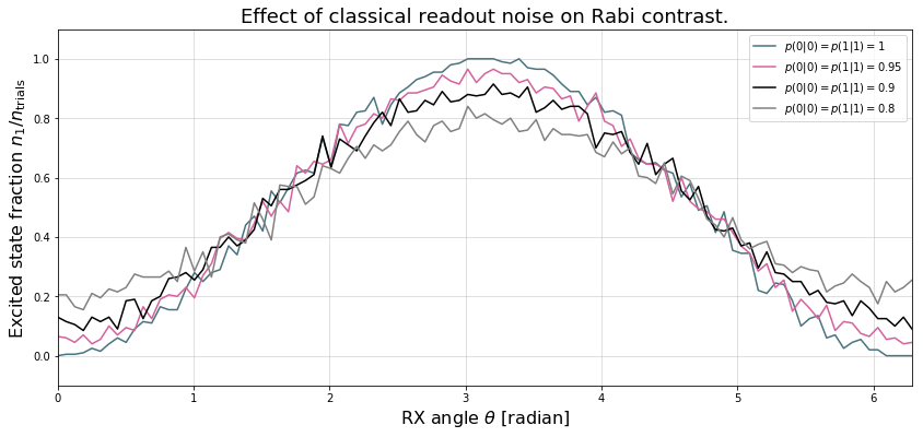
Example 1: Rabi sequence with noisy readout
# number of angles
num_theta = 101

# number of program executions
trials = 200

thetas = np.linspace(0, 2*np.pi, num_theta)

p00s = [1., 0.95, 0.9, 0.8]

results_rabi = np.zeros((num_theta, len(p00s)))

for jj, theta in enumerate(thetas):
    for kk, p00 in enumerate(p00s):
        qc.qam.random_seed = 1
        p = Program(RX(theta, 0)).wrap_in_numshots_loop(trials)
        # assume symmetric noise p11 = p00
        p.define_noisy_readout(0, p00=p00, p11=p00)
        ro = p.declare("ro", "BIT", 1)
        p.measure(0, ro[0])
        res = qc.run(p).get_register_map().get("ro")
        results_rabi[jj, kk] = np.sum(res)
CPU times: user 1.2 s, sys: 73.6 ms, total: 1.27 s
Wall time: 3.97 s
plt.figure(figsize=(14, 6))
for jj, (p00, c) in enumerate(zip(p00s, [DARK_TEAL, FUSCHIA, "k", "gray"])):
    plt.plot(thetas, results_rabi[:, jj]/trials, c=c, label=r"$p(0|0)=p(1|1)={:g}$".format(p00))
plt.legend(loc="best")
plt.xlim(*thetas[[0,-1]])
plt.ylim(-.1, 1.1)
plt.grid(alpha=.5)
plt.xlabel(r"RX angle $\theta$ [radian]", size=16)
plt.ylabel(r"Excited state fraction $n_1/n_{\rm trials}$", size=16)
plt.title("Effect of classical readout noise on Rabi contrast.", size=18)
print(plt)
<matplotlib.text.Text at 0x104314250>
Example 2: Estimate the assignment probabilities
Here we will estimate \(P_{x'|x}\) ourselves! You can run some simple experiments to estimate the assignment probability matrix directly from a QPU.
On a perfect quantum computer
print(estimate_assignment_probs(0, 1000, qc))
[[1. 0.]
 [0. 1.]]
On an imperfect quantum computer
qc.qam.random_seed = None
header0 = Program().define_noisy_readout(0, .85, .95)
header1 = Program().define_noisy_readout(1, .8, .9)
header2 = Program().define_noisy_readout(2, .9, .85)

ap0 = estimate_assignment_probs(0, 10000, qc, header0)
ap1 = estimate_assignment_probs(1, 10000, qc, header1)
ap2 = estimate_assignment_probs(2, 10000, qc, header2)
print(ap0, ap1, ap2, sep="\n")
readout-noise

[[ 0.84967  0.04941]
 [ 0.15033  0.95059]]
[[ 0.80058  0.09993]
 [ 0.19942  0.90007]]
[[ 0.90048  0.14988]
 [ 0.09952  0.85012]]
Example 3: Correct for Noisy Readout
Correcting the rabi signal from above
ap_last = np.array([[p00s[-1], 1 - p00s[-1]],
                    [1 - p00s[-1], p00s[-1]]])
corrected_last_result = [correct_bitstring_probs([1-p, p], [ap_last])[1] for p in results_rabi[:, -1] / trials]
plt.figure(figsize=(14, 6))
for jj, (p00, c) in enumerate(zip(p00s, [DARK_TEAL, FUSCHIA, "k", "gray"])):
    if jj not in [0, 3]:
        continue
    plt.plot(thetas, results_rabi[:, jj]/trials, c=c, label=r"$p(0|0)=p(1|1)={:g}$".format(p00), alpha=.3)
plt.plot(thetas, corrected_last_result, c="red", label=r"Corrected $p(0|0)=p(1|1)={:g}$".format(p00s[-1]))
plt.legend(loc="best")
plt.xlim(*thetas[[0,-1]])
plt.ylim(-.1, 1.1)
plt.grid(alpha=.5)
plt.xlabel(r"RX angle $\theta$ [radian]", size=16)
plt.ylabel(r"Excited state fraction $n_1/n_{\rm trials}$", size=16)
plt.title("Corrected contrast", size=18)
print(plt)
<module 'matplotlib.pyplot' from ...>

We find that the corrected signal is fairly noisy (and sometimes exceeds the allowed interval \([0,1]\)) due to the overall very small number of samples \(n=200\).
Corrupting and correcting GHZ state correlations
In this example we will create a GHZ state \(\frac{1}{\sqrt{2}}\left[\left|000\right\rangle + \left|111\right\rangle \right]\) and measure its outcome probabilities with and without the above noise model. We will then see how the Pauli-Z moments that indicate the qubit correlations are corrupted (and corrected) using our API.
ghz_prog = Program(
    Declare("ro", "BIT", 3),
    H(0), CNOT(0, 1), CNOT(1, 2),
    MEASURE(0, ("ro", 0)), MEASURE(1, ("ro", 1)), MEASURE(2, ("ro", 2)),
)
ghz_prog.wrap_in_numshots_loop(10000)
print(ghz_prog)
results = qc.run(ghz_prog).get_register_map().get("ro")
DECLARE ro BIT[3]
H 0
CNOT 0 1
CNOT 1 2
MEASURE 0 ro[0]
MEASURE 1 ro[1]
MEASURE 2 ro[2]
header = header0 + header1 + header2
noisy_ghz = header + ghz_prog
noisy_ghz.wrap_in_numshots_loop(10000)
print(noisy_ghz)
noisy_results = qc.run(noisy_ghz).get_register_map().get("ro")
DECLARE ro BIT[3]
PRAGMA READOUT-POVM 0 "(0.85 0.050000000000000044 0.15000000000000002 0.95)"
PRAGMA READOUT-POVM 1 "(0.8 0.09999999999999998 0.19999999999999996 0.9)"
PRAGMA READOUT-POVM 2 "(0.9 0.15000000000000002 0.09999999999999998 0.85)"
H 0
CNOT 0 1
CNOT 1 2
MEASURE 0 ro[0]
MEASURE 1 ro[1]
MEASURE 2 ro[2]
Uncorrupted probability for \(\left|000\right\rangle\) and \(\left|111\right\rangle\)
probs = estimate_bitstring_probs(results)
print(probs[0, 0, 0], probs[1, 1, 1])
0.50419999999999998 0.49580000000000002
As expected the outcomes 000 and 111 each have roughly
probability \(1/2\).
Corrupted probability for \(\left|000\right\rangle\) and \(\left|111\right\rangle\)
noisy_probs = estimate_bitstring_probs(noisy_results)
print(noisy_probs[0, 0, 0], noisy_probs[1, 1, 1])
0.30869999999999997 0.3644
The noise-corrupted outcome probabilities deviate significantly from their ideal values!
Corrected probability for \(\left|000\right\rangle\) and \(\left|111\right\rangle\)
corrected_probs = correct_bitstring_probs(noisy_probs, [ap0, ap1, ap2])
print(corrected_probs[0, 0, 0], corrected_probs[1, 1, 1])
0.50397601453064977 0.49866843912900716
The corrected outcome probabilities are much closer to the ideal value.
Estimate \(\langle Z_0^{j} Z_1^{k} Z_2^{\ell}\rangle\) for \(jkl=100, 010, 001\) from non-noisy data
We expect these to all be very small
zmoments = bitstring_probs_to_z_moments(probs)
print(zmoments[1, 0, 0], zmoments[0, 1, 0], zmoments[0, 0, 1])
0.0083999999999999631 0.0083999999999999631 0.0083999999999999631
Estimate \(\langle Z_0^{j} Z_1^{k} Z_2^{\ell}\rangle\) for \(jkl=110, 011, 101\) from non-noisy data
We expect these to all be close to 1.
print(zmoments[1, 1, 0], zmoments[0, 1, 1], zmoments[1, 0, 1])
1.0 1.0 1.0
Estimate \(\langle Z_0^{j} Z_1^{k} Z_2^{\ell}\rangle\) for \(jkl=100, 010, 001\) from noise-corrected data
zmoments_corr = bitstring_probs_to_z_moments(corrected_probs)
print(zmoments_corr[1, 0, 0], zmoments_corr[0, 1, 0], zmoments_corr[0, 0, 1])
0.0071476770049732075 -0.0078641261685578612 0.0088462563282706852
Estimate \(\langle Z_0^{j} Z_1^{k} Z_2^{\ell}\rangle\) for \(jkl=110, 011, 101\) from noise-corrected data
print(zmoments_corr[1, 1, 0], zmoments_corr[0, 1, 1], zmoments_corr[1, 0, 1])
0.99477496902638118 1.0008376440216553 1.0149652015905912
Overall the correction can restore the contrast in our multi-qubit observables, though we also see that the correction can lead to slightly non-physical expectations. This effect is reduced the more samples we take.
Alternative: A global Pauli error model
The QVM has support for emulating certain types of noise models. One such model is parametric Pauli noise, which is defined by a set of 6 probabilities:
The probabilities \(P_X\), \(P_Y\), and \(P_Z\) which define respectively the probability of a Pauli \(X\), \(Y\), or \(Z\) gate getting applied to each qubit after every gate application. These probabilities are called the gate noise probabilities.
The probabilities \(P_X'\), \(P_Y'\), and \(P_Z'\) which define respectively the probability of a Pauli \(X\), \(Y\), or \(Z\) gate getting applied to the qubit being measured before it is measured. These probabilities are called the measurement noise probabilities.
We can instantiate a QVM, then specify these probabilities.
# 20% chance of a X gate being applied after gate applications and before measurements.
noisy_qc = get_qc("1q-qvm")
noisy_qc.qam.gate_noise=(0.2, 0.0, 0.0)
noisy_qc.qam.measurement_noise=(0.2, 0.0, 0.0)
We can test this by applying an \(X\)-gate and measuring. Nominally,
we should always measure 1.
p = Program(
    Declare("ro", "BIT", 1),
    X(0),
    MEASURE(0, ("ro", 0)),
).wrap_in_numshots_loop(10)

qc = get_qc("1q-qvm")
print("Without Noise:")
print(qc.run(p).get_register_map().get("ro"))
print("With Noise:")
print(noisy_qc.run(p).get_register_map().get("ro"))
Without Noise:
[[1]
 [1]
 [1]
 [1]
 [1]
 [1]
 [1]
 [1]
 [1]
 [1]]
With Noise:
[[0]
 [1]
 [0]
 [1]
 [1]
 [0]
 [1]
 [1]
 [0]
 [1]]